hashkat.org

The Agent Follow Model

The agent follow_model is one in which agents follow another agent based on that agent's type, though whom they follow within that agent_type is random. That is, an agent may prefer to follow a 'Celebrity' but which celebrity is left to chance. This is a refinement of the random follow_model.

This tutorial should take approximately 10 minutes to complete.

Constructing The Network

We start with the INFILE.yaml file from Tutorial 4 and save it to /hashkat/docs/tutorial_input_files/tutorial05/INFILE.yaml.

In INFILE.yaml we change the parameters to:

• follow model: agent
• 'Celebrity' add: 100.0
• 'Celebrity' follow_rate: 90.0
• 'Standard' follow_rate: 10.0

Observe that both 'Standard' agent_types and 'Celebrity' agent_types have an add weight of 100.0. #k@ will sum the add_weights and divide, so that the simulation will add new agents in the proportion of 50% 'Standard' (100/200) and 50% 'Celebrity' (approximately).

Since celebrities tend to garner vastly more followers than ordinary people, it makes sense for our simulation of 'Standard' and 'Celebrity' agents to mimic this. Therefore, we will change the 'Standard' follow_weight to 10.0 and the 'Celebrity' follow_weight to 90.0. From this we should expect 'Celebrity' agents to garner about 90/100 of the new follows and 'Standard' agents to garner about 10%.

The code is as follows:

agents:
  - name: Standard
    weights:
                # Weight with which this agent is created
      add: 100.0    # add_weight summed with other agents' add_weights to get proportion of this type added
                # Weight with which this agent is followed in agent follow
      follow: 10.0  # follow rate summed with other agents' follow_weight to get proportion of this type followed
      tweet_type:
        ideological: 1.0
        plain: 1.0
        musical: 1.0
        humorous: 1.0

    followback_probability: 0
    hashtag_follow_options:
      care_about_region: false 
      care_about_ideology: false 
    rates: 
                # Rate for follows from this agent:
        follow: {function: constant, value: 0.01}
                # Rate for tweets from this agent:
        tweet: {function: constant, value: 0.01}

  - name: Celebrity
    weights:

      add: 100.0  
      follow: 90.0
      tweet_type:
        ideological: 1.0
        plain: 1.0
        musical: 1.0
        humorous: 1.0

    followback_probability: 0
    hashtag_follow_options:
      care_about_region: false
      care_about_ideology: false 
    rates:
                # Rate for follows from this agent:
        follow: {function: constant, value: 0.01}
                # Rate for tweets from this agent:
        tweet: {function: constant, value: 0.01}

Note items after # are comments to assist the user and are ignored by the compiler.

Running and Visualizing The Network

Running this simulation we produced the following network, visualized in using open license software Gephi. 'Celebrity' agents are shown as red nodes and 'Standard' agents as blue.

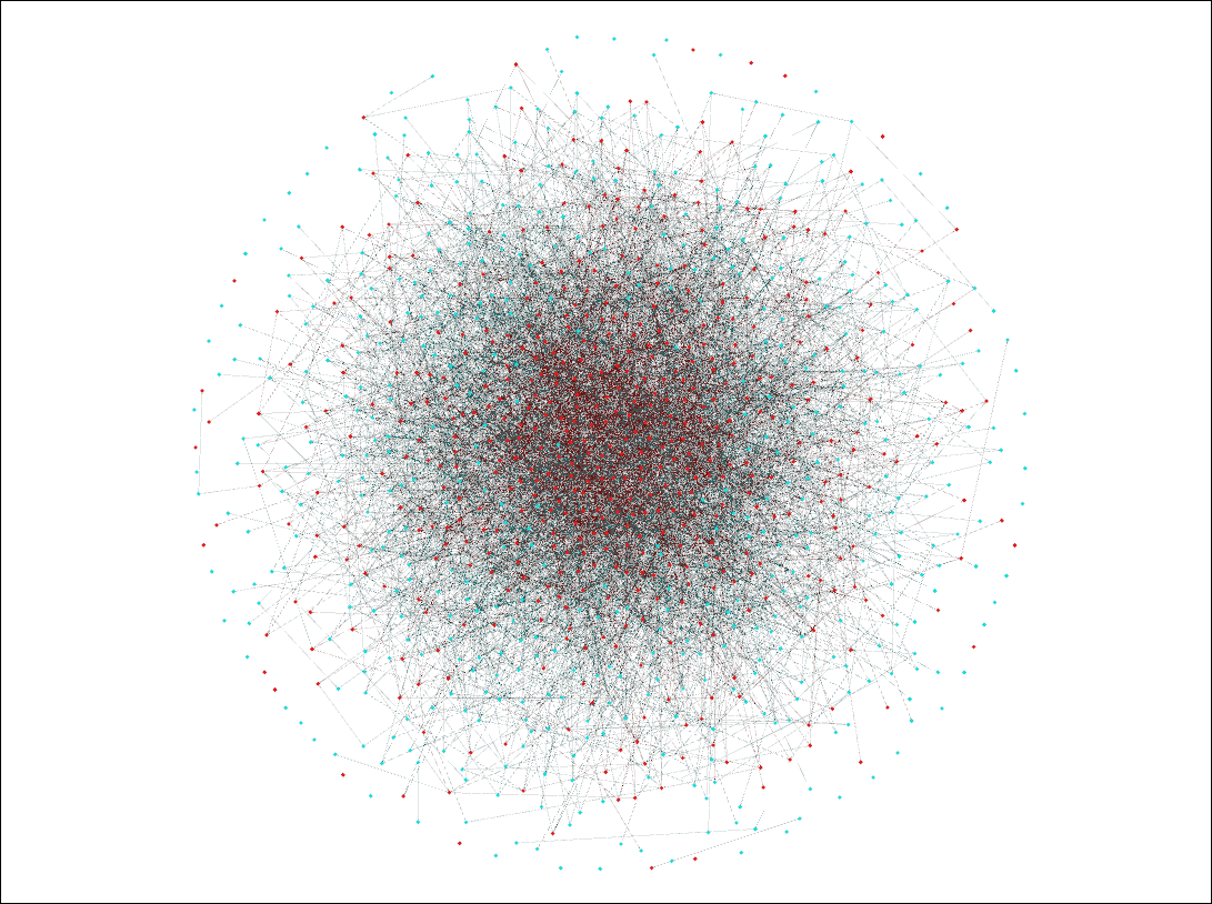
As expected, red nodes are clustered in the center, indicating 'Celebrity' agents have more followers than 'Standard' agents.

We may do further analysis of this network through use of the output files that have been created from running this simulation. As we discussed in Tutorial 1, an agent's cumulative_degree distribution is the total number of connections it has (number of followers and following). We showed how to plot the normalized cumulative_degree distribution probability for all agents in Tutorial 1. Let's do the same here and also compare the overall normalized cumulative_degree distribution to that of each agent type.

We plot the data using open license software Gnuplot with the following commands:

set style fill transparent solid 0.5 noborder

set title 'Cumulative-Degree Distribution'

set xlabel 'Cumulative-Degree'

set ylabel 'Normalized Cumulative-Degree Probability'

plot 'Celebrity_info.dat' u 1:4 lc rgb 'goldenrod' w filledcurves above y1=0 title 'Celebrity', 'Standard_info.dat' u 1:4 lc rgb 'blue' w filledcurves above y1=0 title 'Standard', 'cumulative-degree_distribution_month_000.dat' u 1:2 lc rgb 'dark-red' w filledcurves above y1=0 title 'Overall'

As we can see, there are no 'Standard' agents with a cumulative_degree greater than 20, with most having a cumulative_degree below 10. The 'Celebrity' agents have a higher cumulative_degree distribution, with some 'Celebrity' agents having up to 35 connections in this brief simulation. This would show the role of 'Celebrity' agents in connecting a network.

Next Steps

With the completion of this tutorial you now have some familiarity with the agent follow_model and with networks with more than one agent_type. Adding more agent_types into your simulation, such as 'Bots' and 'Organizations', with different parameters, can lead to some truly complex and interesting networks.

In the next tutorial we combine the twitter_suggest preferential agent follow_model and agent follow_model to create the preferential_agent follow_model, wherein an agent follows another agent based first on agent_type, and second based on which agent, within that type, has the most followers.