Developers

If you are interested in contributing to #k@, please check out the latest build of #k@ at our github repository. If you wish to add any developments to #k@, feel free to do so, and create a pull request, where it will be reviewed and potentially merged in to the hashkat repository. We do ask when modifying #k@, please respect the Google C++ Style Guide.

The source code for #k@ can be found in the src directory. The file ~/hashkat/src/DEVELOPERS.md briefly details the role of every file and directory in the source code.

How Does #k@ Work?

Hashkat is a simulation of a social worker based on agent (node) actions. Actions have a probability of occurring set by the user. At each increment in time, a random number is generated which determines which action is taken.

In #k@ all potential actions have rates. The actions are 'add_agent' (to network), and for each agent 'tweet', 'retweet', 'follow', and 'unfollow'. A further network rate is the 'decay' rate, time after which tweets lose eligibility to be retweeted.

Hashkat takes one action per time increment. Therefore, as the network gets larger, time gets compressed, i.e., if a network with one agent takes an action every hour, a network with 60 agents will take an action every minute, and a network with 3600 agents will take an action every second. This example shows time compression which is dependent on the number of agents.

In the kinetic Monte Carlo (KMC) method, KMC modifies the time increment by the cumulative rate function R. Let me explain. The way the system tracks all the potential actions that can be taken at a given point in time is by the culmulative rate function R, the sum of all the rates within the system. In broad terms, the R function is the sum of the network 'add' rate, and the different agents' 'tweet','follow', and 'retweet' rates:

For n number of agents_types in the system:

R = add_rate + (tweet_rate₁ + follow_rate₁ + retweet_rate₁) + ... + (tweet_rate_n + follow_rate_n + retweet_rate_n)

The default build of #k@ permits 200 different agent_types (n = 200). One may modify the proportions of each agent type, i.e. have 1000 agents of Type 1 (T₁ = 1000), but 10 of Type 2, for a 100:1 ratio T1:T2.

Then the R function becomes:

R = add_rate + T₁(tweet_rate₁ + follow_rate₁ + retweet_rate₁) + ... + T_n(tweet_rate_n + follow_rate_n + retweet_rate_n)

Each separate rate is divided by the culmulate rate R, and 'stacked', so that there are a 'spectrum' of actions available in the numerical range 0-1.

Example:

At time₀, there are no agents in the system (n = 0) so the only relevant rate is the add_rate. Let us assume there is a 40% add_rate. This results, at this time, of the chance of an agent being added in the next time increment of 100%.

R = add_rate + 0 + ... + 0 = 40
add_rate/R = 40/40 = 1 => 100% chance of adding an agent

At time₁, there is one agent in the system (n = 1). Agent_1 can tweet, but can't follow or retweet because there are no other agents in system. Let us assume agent_1 has a 10% tweet rate.

R = add_rate + tweet_rate_1
R = 40 + 10
p(new agent will be added) = add_rate/R = 40/50 = 80%
p(agent_1 will tweet) = tweet_rate/R = 10/50 = 20%
add_rate/R = 1 - tweet_rate/R = 1 - 20% = 80%

Thus there is a smaller chance of adding an agent, athough the add rate has not changed.

The 'spectrum' of choices is then:

0.0 -> 0.80 add agent
0.81 -> 1.0 agent_1 tweets.

A random number is generated. If the random number is 0.3 (for example), an agent will be added to the network.

Once the action has been taken, R is recalculated.

With two agents in the system (n = 2), both may follow, both may tweet, and both may retweet, so rates included in R have increased. Let us assume agent_1 has a 4% retweet rate, and a 3% follow rate, and agent_2 has a 15% tweet rate, a 2% retweet rate, and a 6% follow rate.

R = 40 + (10 + 4 + 3) + (15 + 2 + 6) =  80

The spectrum would then be:

0.0 -> 0.49 add agent
0.50 -> 0.625 agent_1 tweets
0.626 -> 0.675 agent_1 retweets
0.676 -> 0.7 agent_1 follows
0.701 -> 0.899 agent_2 tweets
0.9 -> 0.925 agent_2 retweets
0.925 -> 1.0 agent_2 follows

A random number is generated. Let us assume that number is 0.76. Then the action taken is that agent_2 tweets. At this point R recalculated, time increments, and the cycle repeats. As we can see R increases rapidly.

Time Compression

As the absolute value of R increases (in our example it has gone from 40 to 80), time compresses.

If use_random_time_increment in INFILE.yaml is enabled, a different random number r_t is generated, and time will move forward by:

Δt = -log(r_t) / R

If it is not enabled, time will move forward by:

Δt = 1 / R

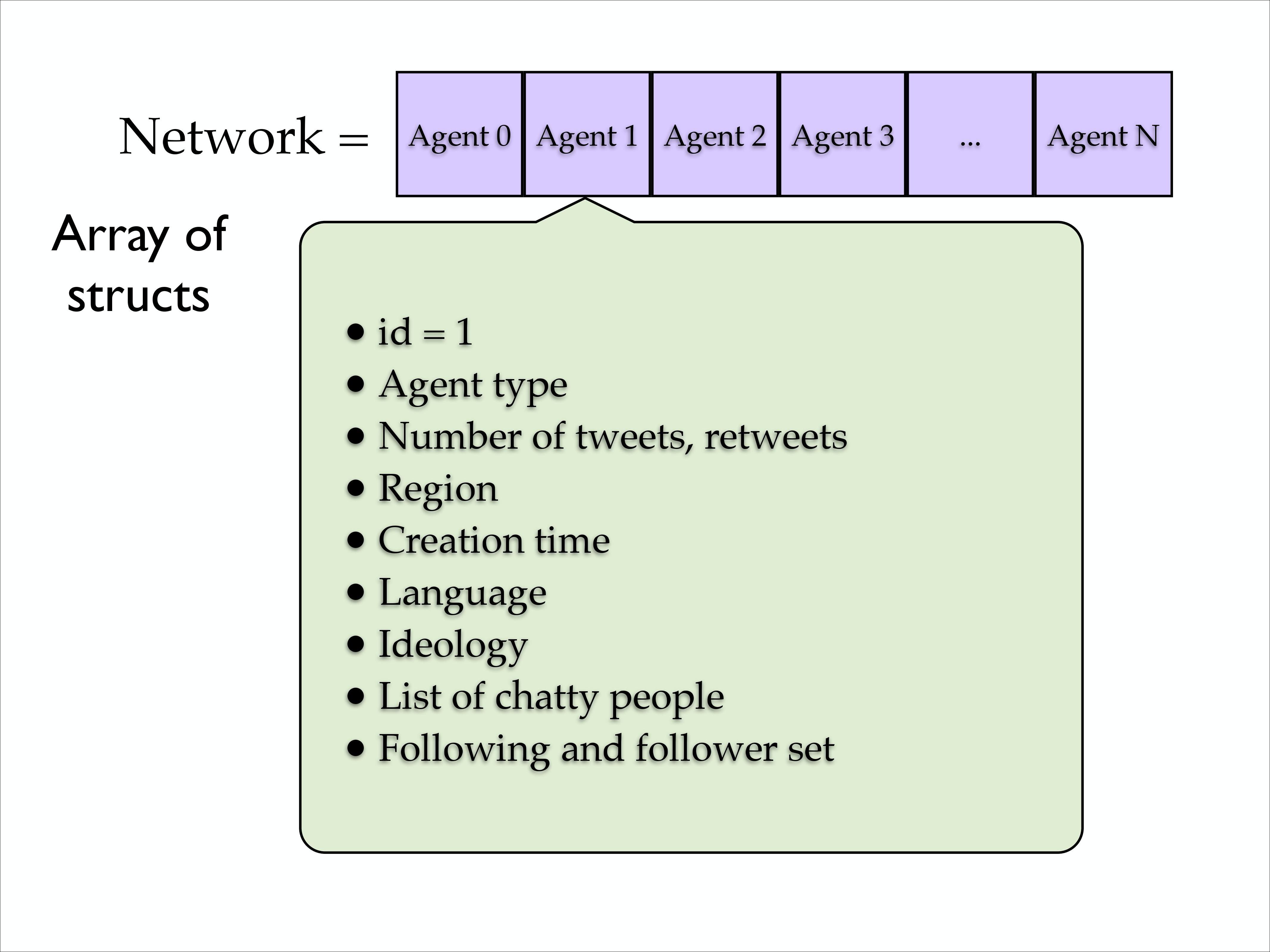
Network

In terms of programming, the network is an array of agent structs as shown.

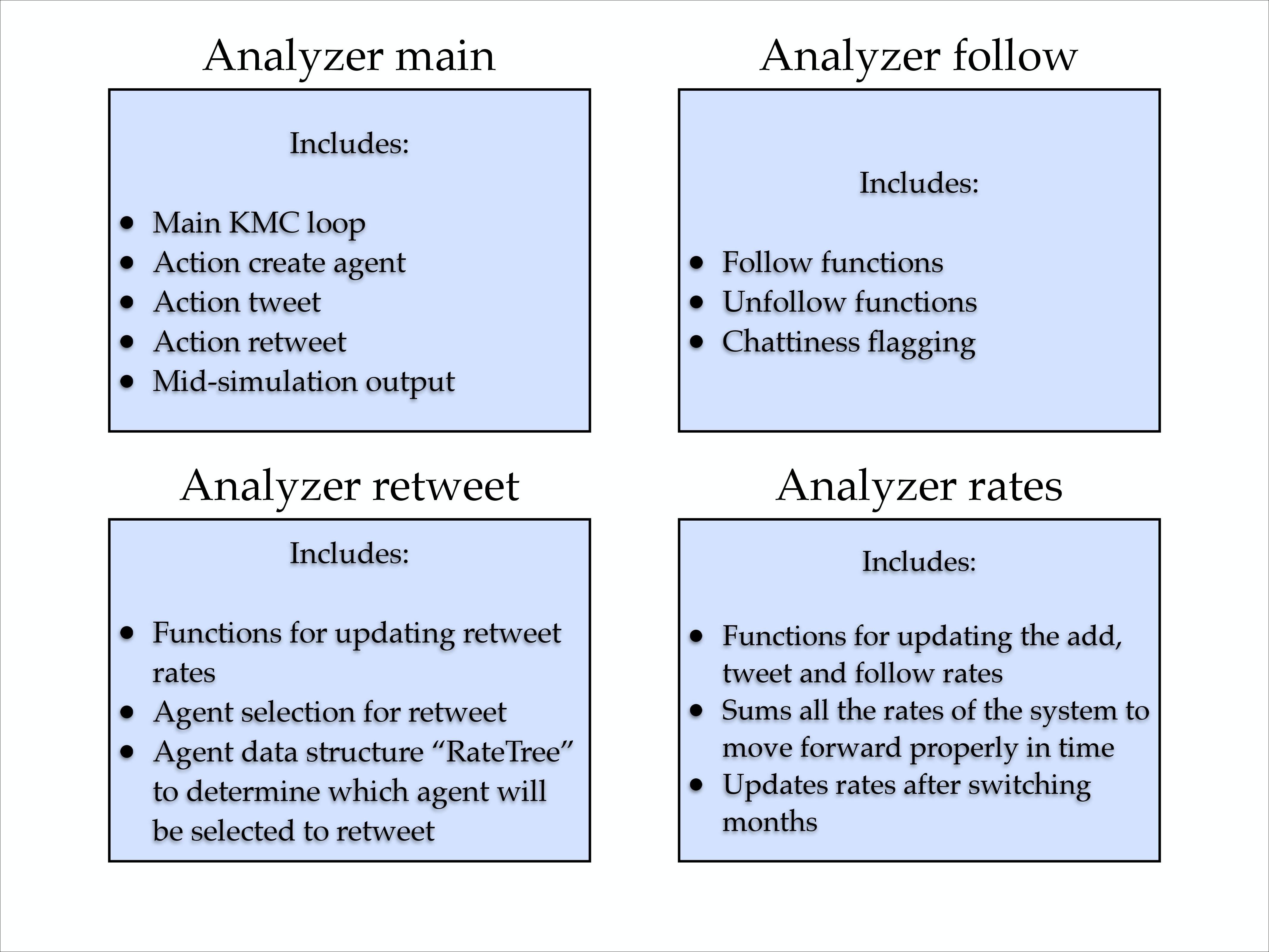
Analyzer Files

Keeping track of all the potential actions (rates) in the system and implementing the chosen action properly is vital. Four very important 'Analyzer' files in the source code are summarized below:

Simulation Workflow

The concept map below gives a brief summary of how #k@ runs.

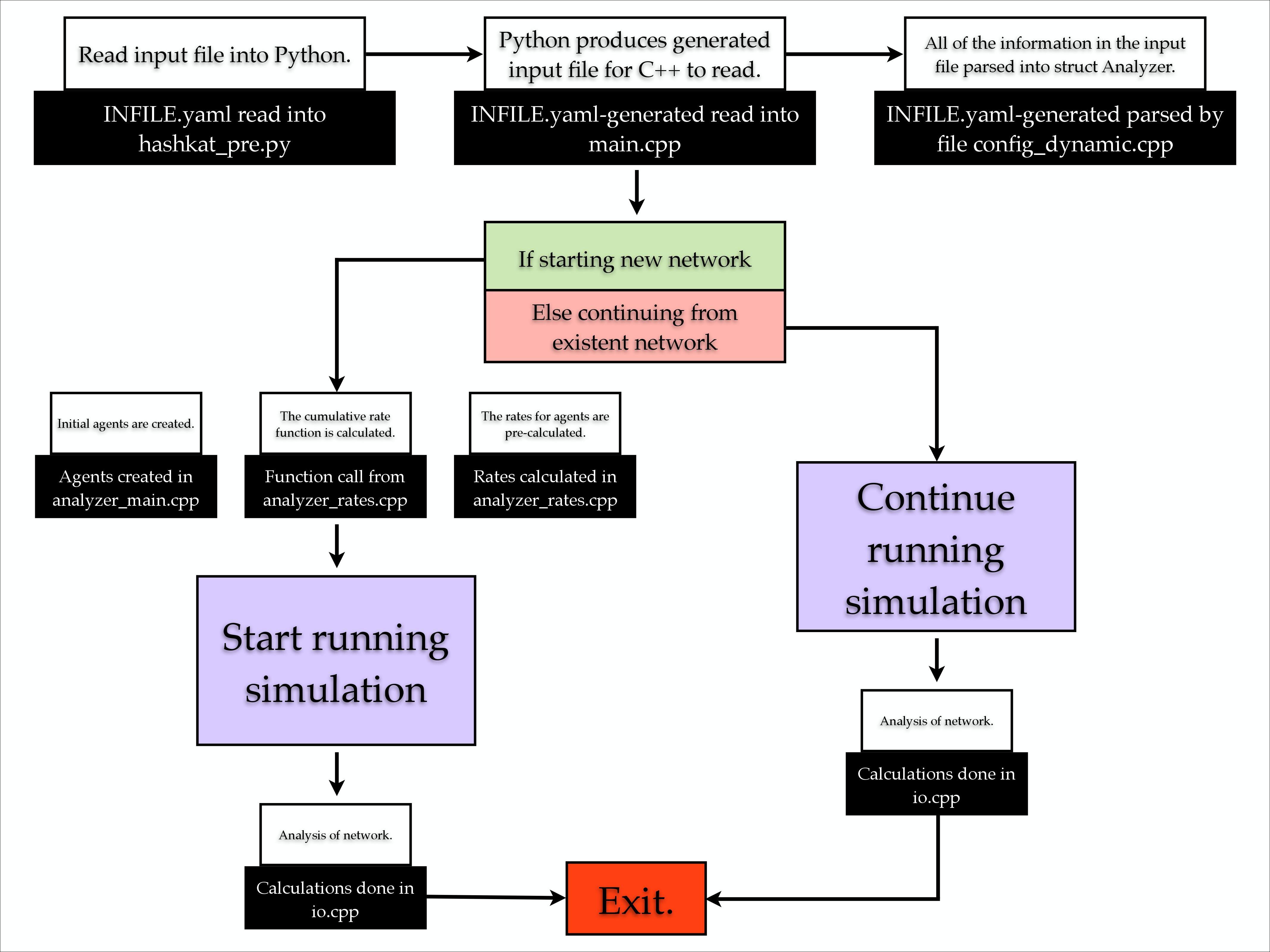
The input file INFILE.yaml is configured, then read into Python via hashkat_pre.py. Python then generates an input file INFILE.yaml-generated for C++ to read in the main.cpp file. From there the information from the input file is put into the 'Analyzer' structure by parsing INFILE.yaml-generated into config_dynamic.cpp while one of the following occurs:

if starting a new network, the initial agents are created in analyzer_main.cpp while agent rates and the cumulative rate function are calculated in analyzer_rates.cpp prior to the start of the network simulation; the simulation then runs, and analysis of the network simulation is done in io.cpp. The simulation then finishes and exits.
if continuing an existing network, the simulation will continue running with analysis done in io.cpp. The simulation then finishes and exits.

Code Map

The rates in #k@ are: 'add', 'follow', 'unfollow', 'tweet' and 'retweet'. The code map below outlines how rates work.

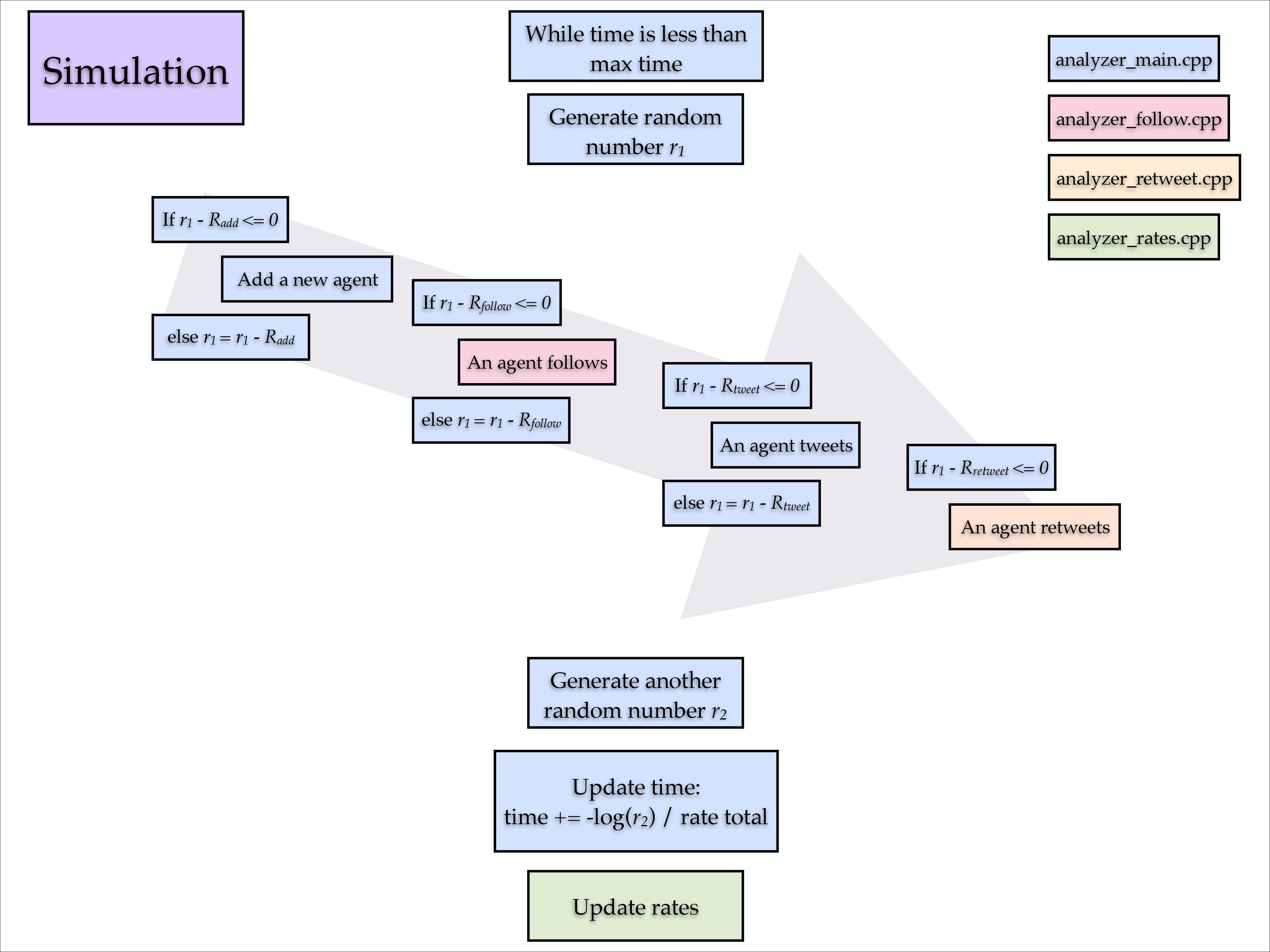
In brief, in analyzer_main.cpp, if the simulated time and real time elapsed are less than maximum simulated and real time allotted, a random number, r, is generated. The first is r is r₁.

If r₁ and the normalized 'add' rate have a difference less than or equal to zero, a new agent is 'added' to the network.
If this is not the case, the value of r₁ is decreased by the normalized 'add' rate.
If r₁'s new value and the normalized 'follow' rate have a difference less than or equal to zero, an agent 'follows' another agent via analyzer_follow.cpp.
If this is not the case, the value of r₁ is decreased by the normalized 'follow' rate.
If r₁'s new value and the normalized 'tweet' rate have a difference less than or equal to zero, an agent 'tweets'.
If this is not the case, the value of r₁ is decreased by the normalized 'tweet' rate.
If r₁'s new value and the normalized 'retweet' rate have a difference less than or must be less than or equal to zero, an agent 'retweets' via analyzer_retweet.cpp.
If 'use_random_time_increment' is enabled, the simulated time moves forward by:

t += -log(r_t) / R
If 'use_random_time_increment' is disabled, the simulated time moves forward by:

t += 1 / R

where R is the cumulative rate function, the sum of all the rates.

Once this is completed, another random number, r₂ is generated.

The process repeats until the maximum real or simulated time is reached.

Hashkat in Action

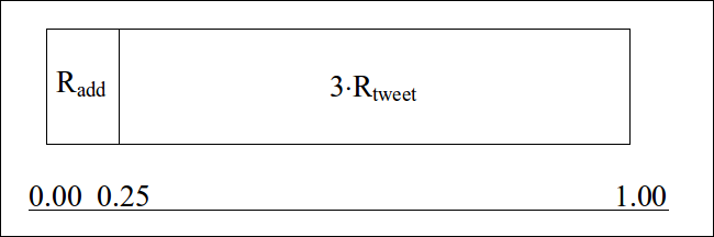
Another description of how rates work in #k@ is as follows. We initially have one agent (n = 1) in the network, with agent 'add' rate set to 1 agent per simulated minute (R_add = 1) and agent 'tweet' rate set to 1 tweet per simulated minute (R_tweet = 1). We've ignored the 'follow' and 'retweet' rates in this example.

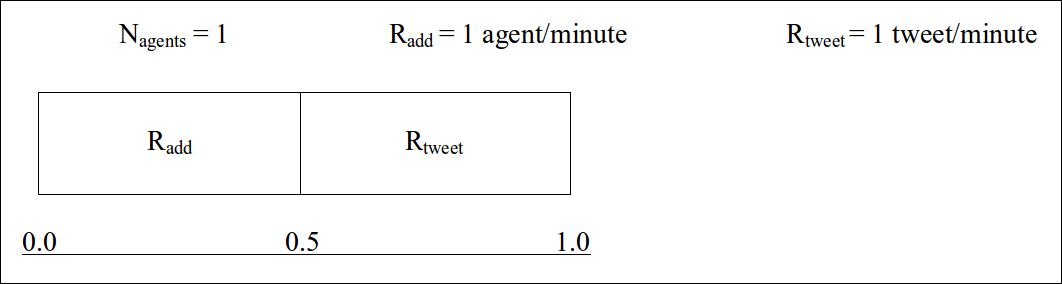
At start there is a 1/2 chance that another agent will be added to the network and 1/2 chance the initial agent will make a tweet. A random number is generated. If the random number is less than or equal to 0.5, another agent will be added, if it is greater than 0.5, the initial agent will tweet. Time will then move forward.

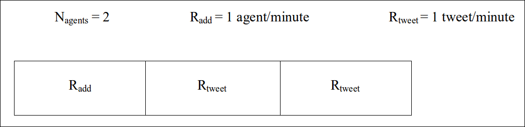
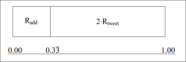
Let's say that another agent has been added to the network (n = 2). The chance of 'add' becomes 1/3 and chance of a tweet becomes 2/3. The chance of an agent tweeting is now twice as likely as a new agent being added in the KMC loop. It should be noted that the expected output of each agent will remain the same since the simulated time will move more slowly due to time being inversely proportional to the increasing cumulative rate function (R).

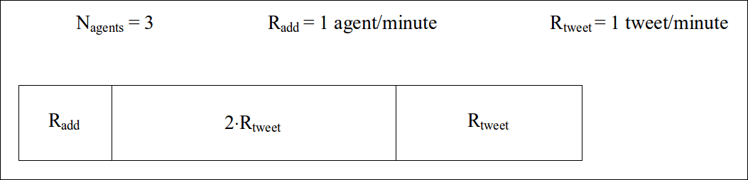
Let's add an additional agent to the network (n = 3). There is now a 1/4 chance of an 'add' and a 3/4 chance of a 'tweet'.

This cycle will continue until real or simulated time elapsed reaches the maximum alloted.

This is the kinetic Monte Carlo (KMC) method in #k@.

Build Tests

Build tests can be run in #k@ by running the tests.sh script. This script runs network simulations using the input files found in ~/hashkat/tests/referencefiles/, and compares the output of these files to expected output using the verify.py script. If there are any discrepancies between the data of a particular output file and its corresponding reference data, the file for that particular test is printed to the screen.