The Random Follow Model
Follow_models simulate how agents chose to follow other agents. There are six different follow_models in #k@. Each of the follow models will be discussed in its own tutorial. The input data used to create the networks will be almost the same for each follow model tutorial so that the results may be easily compared. This tutorial should take approximately 20 minutes to complete.
The six k#@ follow models are:
- Random
- Twitter_Suggest (Preferential_Global)
- Agent
- Preferential_Agent
- Hashtag
- Twitter (Combination)
In the random follow_model the agent's choice of whom to follow is arbitrary or random. Our model is based on the work of Paul Erdos & Alfred Renyi. The network we created in Tutorial 1 used the random follow model.
In this tutorial we start configuring the input file to show you how to create a network to your specifications. The file for configuration is INFILE.yaml. The file we create in this tutorial may be found at hashkat/docs/tutorial_input_files/tutorial03.
For more information on configuration see the Input and Output pages.
Constructing The Network
This simulation will be succinct. We start with Tutorial 1's INFILE.yaml. If we have not changed the parameter it may not be shown.
For this tutorial set:
- (rates subsection) add: 0
- initial_agents: 1000
- max_agents: 1000
- max_simulated_time: 1000
- max_real_time: 1
- max_analysis_steps: unlimited
- enable_interactive_mode: false (off), therefore enable_lua_hooks: false, and the lua_script setting will be ignored.
- use_barabasi: false, therefore barabasi_connections will be ignored by the compiler.
- barabasi_exponent: 1
- randome_time_increment: true
- follow_model: random
- stage1_unfollow: false
- unfollow_tweet_rate: 10000
- use_hashtag_probability: 0.5
We will discuss Barabasi options in Tutorial 4.
Model_weights are only necessary for the twitter follow_model, shown in Tutorial 8, and will be ignored but we show them here, set at 0, to introduce them.
To turn off the 'unfollow_tweet_rate' we set it to an exceptionally high number (i.e. 10,000 per minute). An agent would have to send 10,000 tweets a minute for another agent to unfollow them.. We have set the chance of a hashtag in a tweet at 50%.
The code looks like this:
analysis:
  initial_agents:
    1000
  max_agents:
    1000
  max_time:
    1000
  max_analysis_steps:
    unlimited
  max_real_time:
    1
  enable_interactive_mode:
    false
  enable_lua_hooks: # only compiled when enable_interactive_mode: true
    false
  lua_script:   # only compiled when enable_interactive_mode: true
    INTERACT.lua
  use_barabasi:
    false
  barabasi_connections: # only compiled when use_barabasi: true
    100
  barabasi_exponent:
    1
  use_random_time_increment:
    true
  use_followback:
    false
  follow_model:
    random
  model_weights: {random: 0.0, twitter_suggest: 0.0, agent: 0.0, preferential_agent: 0.0, hashtag: 0.0}
        # model weights are ONLY necessary for follow_method 'twitter' (combination)
  stage1_unfollow:
    false
  unfollow_tweet_rate:
    10000
  use_hashtag_probability:
    0.5
Note items after # are comments to assist the user and are ignored by the compiler.
In the 'rates' subsection of INFILE.yaml we set the add_rate to 0. this applies to the network as a whole. We will only use one type of agent, 'Standard', so that agent's add rate is 100.0 (all new agents will be 'Standard'). The 'Celebrity' agent_type is named but not added ('add: 0'). 'Celebrity' agents will be used in Tutorial 5 and onward.
We leave the the output section of INFILE.yaml as in Tutorial 1. The tweet and retweets rates are as in Tutorial 1, 1 per 100 simulated minutes. The follow_ranks_threshold and weight entries, Ideologies and Regions sections have also remained the same.
agents:
  - name: Standard
    weights:
      add: 100.0        # Weight with which this agent is created
      follow: 5     # Weight with which this agent is followed in agent follow
      tweet_type:
        ideological: 1.0
        plain: 1.0
        musical: 1.0
        humorous: 1.0
    followback_probability: 0   # Probability that following this agent results in a follow-back
    hashtag_follow_options:
      care_about_region: false  # does the agent care about where the agent they will follow is from?
      care_about_ideology: false  # does the agent care about the ideology of the agent they will follow?
    rates:
        follow: {function: constant, value: 0.01}  # Rate for follows from this agent:
        tweet: {function: constant, value: 0.01}  # Rate for follows from this agent:

  - name: Celebrity
    weights:
      add: 0
      follow: 5
      tweet_type:
        ideological: 1.0
        plain: 1.0
        musical: 1.0
        humorous: 1.0
    followback_probability: 0
    hashtag_follow_options:
      care_about_region: false
      care_about_ideology: false
    rates:
        follow: {function: constant, value: 0.01}
        tweet: {function: constant, value: 0.01}
We have added the 'Celebrity' agent_type to our input file by copying the 'Standard" agent_type and renaming it. We will not be adding this agent_type until Tutorial 4 ('add: 0') so configuration can be done later. We have changed the 'Standard' followback_probability to 0, though this is irrelevant since we have use_followback set to 'false'. This is to give consistency to later tutorials.
Running and Visualizing The Network
The video below shows you how to save, run and then visualize the output using open license software Gephi.
In Gephi we produce a network similar to the one shown below:
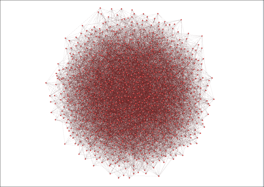
This a random network, with no clear agent or group of agents being the most popular.
Plotting Network Output
To plot the data produced by our simulation, we use open license software Gnuplot.
Let us take the example of the culmulative_degree of an agent. With agents having a follow rate of 1/100 per simulated minute, in a simulation 1000 sim_minutes long, we would expect most agents to have an in_degree of 10 (ten people following them), and an out_degree of 10 (10 people they follow) for a cumulative_degree distribution of 20.
Let's plot this distribution using Gnuplot, with data points instead of filled curves. In Gnuplot the commands to do this are:
set title 'Cumulative-Degree Distribution'
set xlabel 'Cumulative-Degree'
set ylabel 'Normalized Cumulative-Degree Probability'
plot 'cumulative-degree_distribution_month_000.dat' title ''
Giving us:

As we can see, there is a definite peak surrounding 20 degrees, though it seems that more agents happen to have a cumulative-degree just below or just above 20 for this simulation.
To run the EXACT SAME simulation again, remove the output files network_state.dat and output directory from this simulation and run it again. It will give the same output because the same seed for the random number generator will be used.
Running a Network Simulation with a Random Seed
To run a network simulation and obtain a different output each time you need to use a random seed for the random number generator. To use a random seed, run the program with this command:
./run.sh --rand
Running this network simulation multiple times, each time using './run.sh --rand', we produced the following cumulative_degree distribution plot:

As we can see, the cumulative_degree distribution of the random follow model matches the Poisson Distribution.
To create this plot, we ran three simulations with random seeds and renamed their cumulative_degree distributions as:
- cumulative-degree_distribution_month_000.a
- cumulative-degree_distribution_month_000.b
- cumulative-degree_distribution_month_000.c
We entered the following in Gnuplot:
poisson( x , mu ) = exp(-mu) * mu**(x) / gamma(x+1)
set xrange [0:50]
set title 'Cumulative-Degree Distribution for Simulations with Different Seeds'
set xlabel 'Cumulative-Degree'
set ylabel 'Normalized Cumulative-Degree Probability'
plot poisson( x , 20 ) title 'Poisson Distribution',
'cumulative-degree_distribution_month_000.a' title '',
'cumulative-degree_distribution_month_000.b' title '',
'cumulative-degree_distribution_month_000.c' title ''
Your output will vary.
Next Steps
Try running your own random follow model simulation that is different from the one outlined above, and see what you can create.
When ready, move on to the next tutorial, where things get more interesting with the twitter_suggest follow model.